引
- 在上一讲中我们已经介绍了difussion model是如何定义,如何进行训练的,现在我们可以用flow matching 或者 score matching来训练一个generative model,并且用ODE或者SDE进行采样。但是在真正使用时,我们肯定是希望能够给定一个prompt来进行条件生成的,而我们上述的模型都是直接在$z \in data$上进行训练的,至于最终的采样结果完全是z中一个随机点,所以我们需要一些方法来让我们的模型能够根据一个prompt来进行条件生成。
Vanilla Guidance
我们首先来介绍一下最简单的vanilla guidance方法,定义如下:
$$ \begin{align*} & \textbf{Initialization: } \qquad X_0 \sim p_{\text{init}} \\ & \textbf{Simulation: } \qquad \quad dX_t = u_t^\theta(X_t \mid y) \, dt + \sigma_t \, dW_t \\ & \textbf{Goal: } \qquad \qquad \qquad X_1 \sim p_{\text{data}}(\cdot \mid y) \end{align*} $$当这里的$\sigma_t = 0$时,我们称之为guided flow model, 我们接下来谈谈如何在guided flow model中进行训练。一个很简单的想法就是在原先的训练方式上我们就加上一个y的限制,其他都不变: 给定一个prompt y, 我们就从$z \in p_{data}(\cdot|y)$中sample一个z, 然后按照之前的方式从$z$出发进行训练,类似这样:
$$\mathbb{E}_{z \sim p_{\text{data}}(\cdot|y), \, x \sim p_t(\cdot|z)} \left\| u_t^\theta(x \mid y) - u_t^{\text{target}}(x \mid z) \right\|^2$$Note that the label y does not affect the conditional probability path pt(·|z) or the conditional vector field $u_t^{\text{target}}(x|z)$ (although in principle, we could make it dependent). Expanding the expectation over all such choices of y, we thus obtain a guided conditional flow matching objective.
$$\mathcal{L}_{\text{CFM}}^{\text{guided}}(\theta) = \mathbb{E}_{(z,y) \sim p_{\text{data}}(z,y), \, t \sim \text{Unif}[0,1], \, x \sim p_t(\cdot|z)} \left\| u_t^\theta(x|y) - u_t^{\text{target}}(x|z) \right\|^2$$可以注意到这个公式和我们之前定义的flow matching的loss函数非常相似,唯一的区别就是这里是从$p_{data}$中取一个(z,y)对来训练,同时我们的模型接受的输入是(x,y)。
这个方法理论上是可行的,但是实际训练结果证明效果并不好(相关但是不够准确),可能是模型没有学习到正确的marginal vector field, 或者是网络上的(image, text)数据本身有问题。为了强化生成结果和prompt的相关性,我们介绍一种当前SOTA(state-of-the-art)的训练方法。
Classifer-Free Guidance
Classifier Guidance
- 我们首先介绍Classifier Guidance,在gaussian probability path的例子中,我们有vector field和score function之间的一个线性关系,用(x|y)替换后有: $$u_t^{\text{target}}(x|y) = a_t \nabla \log p_t(x|y) + b_t x \tag{1}$$
这里的看似显然的替换值得思考,实际上$p_t(x|y)$和$p_t(x)$是一个东西,后者理解为对所有的$z \in data$进行一个加权,前者也可以看成是对所有的$z \in data(y)$进行一个加权,只不过前者是后者数据范围的一个子集罢了。于是乎,利用加权积分的线性性质在$z \in data(y)$上展开一次就得证了。
对于prompt下的概率路径$p_t(x|y)$, 我们有:
$$p_t(x|y) = \frac{p_t(x) p_t(y|x)}{p_t(y)}$$进一步有:(where we used that the gradient $\nabla$ is taken with respect to the variable x, so that $\nabla \log p_t(y) = 0$)
$$ \nabla \log p_t(x|y) = \nabla \log \frac{p_t(x) p_t(y|x)}{p_t(y)} = \nabla \log p_t(x) + \nabla \log p_t(y|x) $$将这个式子代入上面(1)式中,有:
$$u_t^{\text{target}}(x|y) = b_t x + a_t \left( \nabla \log p_t(x) + \nabla \log p_t(y|x) \right) = u_t^{\text{target}}(x) + a_t \nabla \log p_t(y|x)$$这个式子可以看成两部分,第一部分是我们之前的unconditional marginal vector field, 第二部分可以理解为给定x,y分类的score function, 它的作用就是让x更倾向于分类y。之前我们提到使用vanilla guidance方法训练出来的结果不够符合prompt的要求,一个自然的想法就是我们增大第二部分的系数,即:
$$\tilde{u}_t(x|y) = u_t^{\text{target}}(x) + w a_t \nabla \log p_t(y|x), \quad \text{(classifier guidance)}$$where w > 1 is known as the guidance scale.
- How can we learn the term log $p_t(y|x)$? Note that this can be considered as a sort of classifier of noised data (i.e. it gives the log-likelihoods of y given x). So we can simply learn it via supervised learning. 这里的supervised learning的意思应该我们从data中取一对(z,y), 然后在z上加一个噪声,$x = \alpha_t z + \beta_t \epsilon$, 然后让神经网络根据这个x来预测y。
这里有一个细节是,我们用了大量的(z,y)训练一个很好的分类器之后,在第二步训练时我们是对x求解梯度,通过改变x来让它更倾向于分类y!所以我们称这个方法为classifier guidance. 由于这个方法需要额外训练一个分类器模型,需要两倍的工作量,并且当y不是一个类别标签而是一个高维度文本描述时,这个分类器的训练会非常困难,求梯度更是难上加难。
其实,只有当w=1的时候,classifier guidance才是真正的guided vector field, 当w不等于1时,虽然它的采样结果更符合prompt,但是 it is not the “true” guided vector field. (偏离真实vector field,但结果更fit,这就是reinforce)
Classifier-Free Guidance
- 由于上述提到的两个困难,我们需要一个classifier-free guidance的方法。 Classifier-free guidance results in the theoretically equivalent effect as classifier guidance but without having to train a separate classifier.
- 我们利用这个等式: $$\nabla \log p_t(x|y) = \nabla \log p_t(x) + \nabla \log p_t(y|x)$$ 代入之前的$\tilde{u}_t(x|y)$的结果中,有: $$\begin{aligned} \tilde{u}_t(x|y) &= u_t^{\text{target}}(x) + w a_t \nabla \log p_t(y|x) \\ &= u_t^{\text{target}}(x) + w a_t \left( \nabla \log p_t(x|y) - \nabla \log p_t(x) \right) \\ &= u_t^{\text{target}}(x) - \left( w b_t x + w a_t \nabla \log p_t(x) \right) + \left( w b_t x + w a_t \nabla \log p_t(x|y) \right) \\ &= (1-w) u_t^{\text{target}}(x) + w u_t^{\text{target}}(x|y). \end{aligned}$$ 你会发现这个公式也是分为两个部分,第一部分依旧是unguided vector field, 第二部分是guided vector field. 也许你会自然的想到我们可以训练两个vector field神经网络来估计它们,然后加权即可。 Wait , wait , 也许我们只用训练一个网络呢?We may augment our label set with a new, additional ∅ label that denotes the absence of conditioning. We can then treat $u^{target}_t (x) = u^{target}_t (x|∅)$. With that, we do not need to train a separate model to reinforce the effect of a hypothetical classifier. This approach of training a conditional and unconditional model in one (and subsequently reinforcing the conditioning) is known as classifier-free guidance (CFG)!
Note that the construction $\tilde{u}_t(x|y) = (1−w)u^{target}_t (x) + wu^{target}_t (x|y)$, is equally valid for any choice probability path‼️, not just a Gaussian one. When w = 1, it is straightforward to verify that $\tilde{u}_t(x|y) = u^{target}_t (x|y)$. Our derivation using Gaussian paths was simply to illustrate the intuition behind the construction, and in particular of amplifying the contribution of a hypothetical “classifier” $\nabla \log p_t(y|x)$.
Training with Classifier-Free Guidance
由上面的推导,我们现在只需要训练一个神经网络来预测$u^{target}_t(x|y)$即可,但是这里有一个问题:我们从data中取得(z,y)时,y不可能是$\emptyset$, 所以需要人工制造空标签。
$$\mathcal{L}_{\text{CFM}}^{\text{CFG}}(\theta) = \mathbb{E}_{(z,y) \sim p_{\text{data}}(z,y), \; t \sim \text{Unif}[0,1], \; x \sim p_t(\cdot|z), \; y \leftarrow \varnothing \text{ w.p. } \eta} \left\| u_t^\theta(x|y) - u_t^{\text{target}}(x|z) \right\|^2$$其中$y \leftarrow \varnothing \text{ w.p. } \eta$的意思是replace y = $\emptyset$ with probability $\eta$.
可以自行欣赏一下note中的训练伪代码,需要注意的是使用ODE最终前向得到的X1并不 aligned with X1 $\in p_{data}(·|y)$ if we use a weight w>1 (之前提到过 the guided vector field not “true” guided vector field, 故从噪音还原到数据的过程必然偏航), 然而, 从结果上看这个方法更能符合prompt提示。所以说Classifier-free guidance 是一种启发式方法,其有效性主要体现在其优秀的实际结果上。事实上现在的AI生成图片或者视频都高度依赖于$w>=4$的classifier-free guidance!
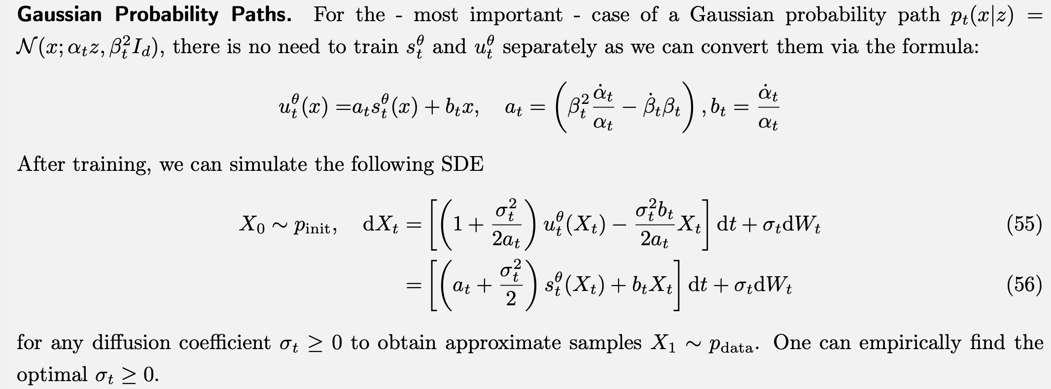
我们上述的讨论都是基于flow model的,对于difussion model来说,如下图所示,利用(55)式将$u^{\theta}_t(X_t)$换成$u^{\theta}_t(X_t|y)$即可进行SDE。